Introduction
So far, we have mostly been working with simple feed-forward neural networks where inputs move through layers sequentially.

For our multilayered perceptrons, these layers have been composed of weights, biases, and activation functions. For our convolutional neural networks, we used convolutional and pooling layers.
Regardless of what these layers were, all of them were feed-forward.
They are trained with backpropagation, but don’t let that confuse you
Feed-forward networks are amazing at some applications, but for applications where previous inputs are significant don’t look anywhere but the simple RNN (we’ll explain this in a bit).
Before we even get started with our RNNs, lets think of why sequences are important in data using a quick thought exercise:
- Recite the alphabet
- Recite the alphabet starting from the letter “K”
- Recite the alphabet backwards
- Tell me the fourteenth letter of the alphabet.
You may have found parts of that challenging. What can this tell you?
You learn the alphabet as a sequence of letters. Sequential memory is a mechanism that makes it easier to recognize these patterns.
What is an RNN?
Suppose we want to create a program that, given a sequence of characters, will predict the next character typed. Why wouldn’t a feed-forward neural network be useful in this case?
Here, the entire sequence of characters is important for predictions, a perfect application of RNNs.
Simply put, an RNN is a neural network that uses sequential memory in a recursive manner. Both inputs and outputs can be sequential. Here are some applications:
| Sequential In | Singular In | |
|---|---|---|
| Sequential Out | Video Summarization | Image Captioning |
| Singular Out | Word Predictor | BOY IF YOU DON’T GIT |
RNN Basics
RNNs use recursive layers in order to consider past inputs.
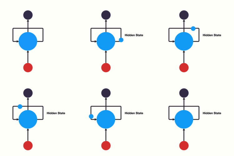
This means that our nodes will eventually consider, to an extent, all previous values in the sequence. If it helps visualize, these layers can be flattened.
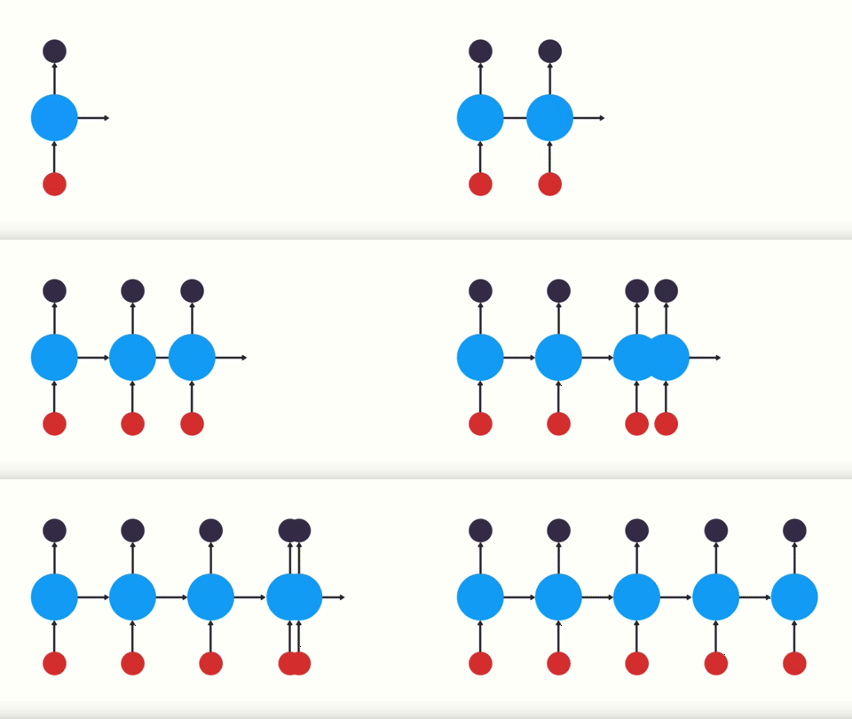
or
In addition to recursive layers, RNNs almost always have feed-forward networks at their tails that help interpret outputs.
The vanishing gradient
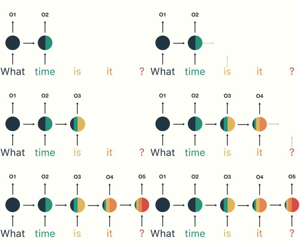
The largest problem with RNNs is the vanishing gradient problem, or the short term memory problem. If you consider our final node, for any RNN, it would look something like this:
 As you can see, the most recent items have the largest impact on the node, while later problems have much smaller presences. This short term memory effect is because of the nature of backpropagation.
To recap, there are three main elements of training deep neural networks:
- Forward-feeding: running our train value up the neural network
- Error: determining the difference between our predicted and labeled values
- “Back Propagation”: running our gradient (delta) down the layers and making changes to Weights and Biases.

The problem here is that each layer makes changes based on the resulting gradient from the previous one. This is our vanishing gradient. This effect is exponential.
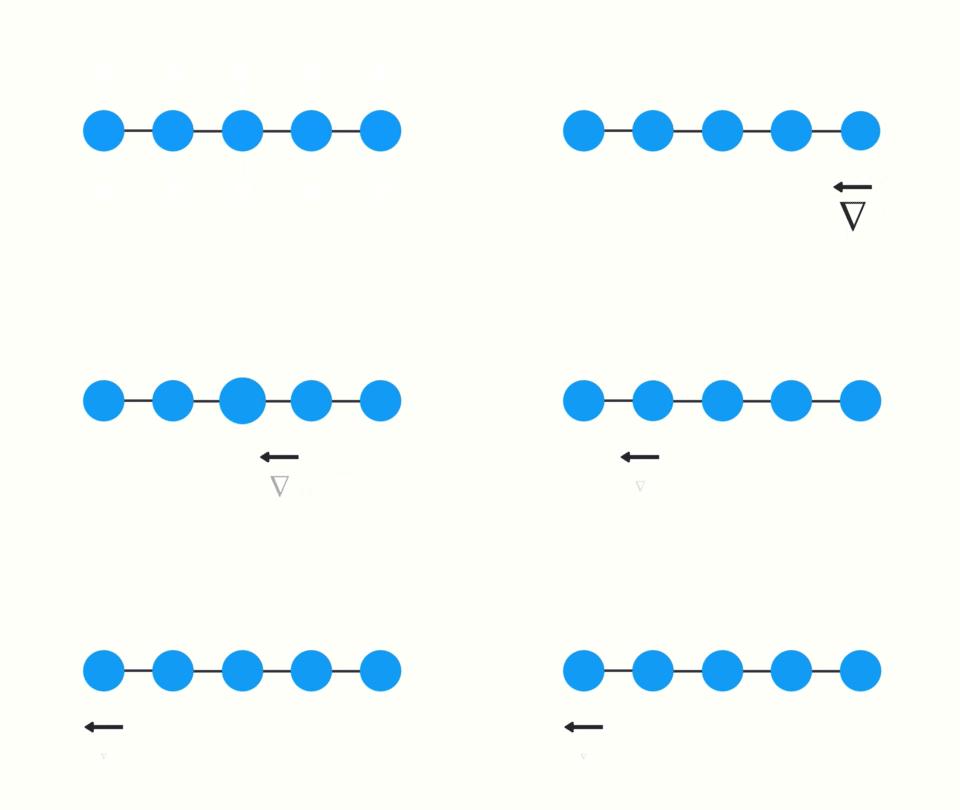
Since our RNNs can be thought of as deep neural nets with variable depth, this effect becomes more of a problem in recursion. If you are predicting the letter following “rosebu…” (it’s a “d”, if you didn’t figure it out yet), short term memory might mean your model is effectively predicting using the three characters “ebu”, which can be fairly ambiguous.
This phenomenon isn’t necessarily a bad thing, rather it’s just how feed-forward NNs are designed. These are the kinds of drawbacks we always hit in machine learning; humans don’t have this vanishing gradient (unless you’re Peter).
Cell architecture
The architecture of the cells within an RNN will determine how it will eventually behave. So far, we have only been working with our standard vanilla cell.
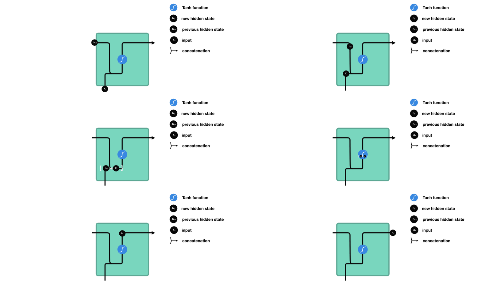
This cell simply combines our previous values, and passes them through a regulating activation function (in this case, $\tanh$). It’s pretty bare bones, which means it’s fast, and can be used in some applications, but it is also very vulnerable to short term memory loss.
Here come LSTMs
LSTMs (“long short-term memory”), along with GRUs (which we won’t go over today), are alternative cell architectures that decide which data within a sequence are most significant (rather than best for last). They use $\tanh$ (-1, 1) and sigmoid (0, 1) activation functions that help determine data that should be forgotten.

The core concept of LSTMs is a cell state, which contains relative information or memory that can be used to determine if data are significant, and the gates. The gates in an LSTM are:
- Input gate: is the cell updated?
- Forget gate: is memory set to zero?
- Output gate: is current cell value made visible?
Let’s go over each of an LSTM’s operations one by one.
[name=Prayag Gordy]uh where?
LSTMs are prone to overfitting, so we’ll also use a concept called “dropout,” a “regularization method where input and recurrent connections to LSTM units are probabilistically excluded from activation and weight updates while training a network.” Essentially, the higher the dropout, the less we overfit; don’t make it too high, however, or you’ll underfit.
Application
There are many applications of RNNs, including:
- Machine translation
- Speech recognition
- Image description
Today, we’ll demo text generation, trained on the book Alice in Wonderland.
