
Implementing XOR
Follow along here.
Prerequisites
Python
A key concept in programming is classes. A class is like a blueprint. It defines the attributes and methods for a type of object.
For example, say we wanted to create a
dogclass. Our dog could have methodsbark()andamIHungry(), and attributesname,barkSound, andhunger.
In order to assign specific values to our object, we create instances.
For example, we can create a member of the
dogclass with “Fido” as thename, “bork bork” as thebarkSound, and 3 as thehunger.
Here is how we could implement this:
class Dog:
    def __init__(self, name, barkSound, hunger):
        self.name = name
        self.sound = sound
        self.hunger = hunger

    def bark(self):
        print(self.sound);

    def amIHungry(self):
        if self.hungerOutOfTen >= 5:
            self.hungerOutOfTen = 0
            print("I was hungry!")
        else:
            print("I'm not hungry.")
Remember that code in Python—unlike in languages like Java—relies on colons and indentation, so make sure to keep your lines organized.
We put self as a method parameter so we can access the attributes of that object. It should always be the first parameter of any method in a Python class.
Now that the Dog class is created, we can create Dog objects.
d1 = Dog("Sparky", "ruff", 8)
d2 = Dog("Fluffy", "woof", 2)

print(d1.name)
d1.amIHungry()

print(d2.name)
d2.amIHungry()
Stupid example, we know, but the applications of classes are endless. If you were to remember only two things, remember that you need an __init__ (that’s two underscores) method, and each method and reference to an attribute must start with self.
The second thing we’ll review is arrays. An array is simply a list of objects; it can be a list of Dog objects, a list of strings, a list of integers—anything.
In the machine learning world, we usually make our arrays with NumPy. The first thing to do when you decide to use NumPy is to import it into the environment using a simple import numpy.
We use NumPy arrays instead of the base arrays because NumPy arrays can handle multiple dimensions.
Some simple ways to create NumPy arrays are below, and more are linked to above.
import numpy as np
a = np.array([2, 3, 1, 0])
b = np.array([[ 1.+0.j, 2.+0.j], [ 0.+0.j, 0.+0.j], [ 1.+1.j, 3.+0.j]]) #what would this create?
A NumPy array has certain attributes: The data type, or dtype, represents the data type of each element; the shape represents the shape of the array (remember matrices?); the size represents the total number of elements; and the number of dimensions, or ndim, can show whether the array is 2D, 3D, etc.
Let’s list the dtype, shape, size, and ndim for b.
Some other important functions we’ll be using from NumPy include:
exp(x)raises todot(array1, array2)calculates the dot product ofarray1andarray2. This is done by multiplying each row ofarray1by each column ofarray2, as we went over in a previous lectureTtransposes an array, in effect reflecting it over the diagonal
Neural Networks
From our last lecture:
Neural networks are comprised of layers. A layer is just a group of neurons. At the front, we have the input layer. The raw data are fed in here. At the end, we have the output layer. This is where the output is displayed.
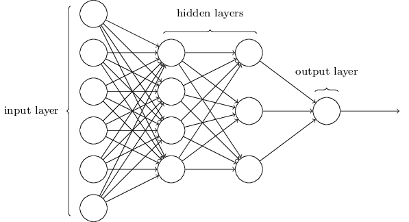
In between are several hidden layers. In these layers, each neuron uses the outputs of the layer before as inputs. The outputs, in turn, are used as the inputs for the next layer. This is how neurons are connected.
Multilayer perceptron neural networks are really just giant composite functions, wherein more layers leads to the multiplication of more weights. These weights are the knobs and dials that allow us to fine-tune our network for the best fit. We use a cost function (remember mean squared error?) to figure out how well our current weights are doing, and then we use gradient descent to change our weights to minimize our error.
And the example of neural networks from the last lecture:
Neural networks allow us to solve problems that other structures can’t. One well-known example is identifying digits.
Suppose we want our neural network to accept images of numbers and to “read” the number. These digits are handwritten, so they vary in size, location, shape, etc.

We could start by considering what our input layer might be. Since the image is comprized of pixels, we can imagine a layer of neurons that each represent a pixel. The shade of the pixel can serve as the value of each neuron.
In the first hidden layer, each neuron will look for an assigned mark. Certain groups of pixels could indicate the presence of the component. The neurons which detect the mark will return a value closer to 1.
The remaining hidden layers will attempt to “assemble” the number. These layers will compile clusters of marks in bigger marks and curbes and, eventually, into loops and lines.
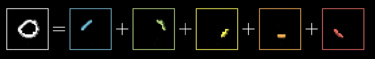
Finally, the output layer would take these biggests parts—loops and lines—and return the predicted number. For example, an upper and lower circle could indicate an eight.
This is what the neural network would look like in action:

Reviewing the Problem
Today, we’ll be tackling the XOR problem. The challenge was to design an algorithm that could correctly classify predict the outcome of a XOR gate.

The XOR gate is simple. The gate accepts two Boolean inputs, A and B, and only returns true if A is not B.

But, simple classifiers won’t work here. For example, if we try to use linear regression, we quickly find out that no line can split the data.
We need an activation function to move from linear fitting to something that works better. We’ll use the sigmoid function, which is shown below:
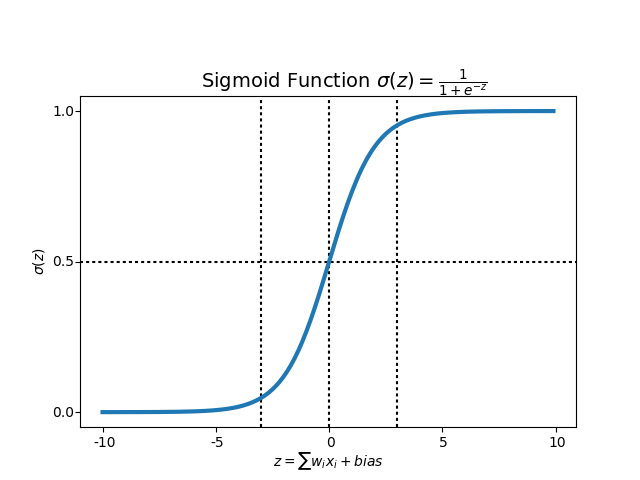
The sigmoid function takes us away from linearity, allowing us to fit our XOR problem.
Starting our Implementation
The first step is to create our NeuronLayer class, where each of its instances represents a layer.
In the __init__ function, we need to initialize the synaptic weights, which represent the strength of the connections between nodes:
from numpy import exp, array, random, dot

class NeuronLayer():
    def __init__(self, number_of_neurons, number_of_inputs_per_neuron):
        # Create Random Weights from [-1, 1) centered at 0
        # What does random.random() do?
        self.synaptic_weights = 2 * random.random((number_of_inputs_per_neuron, number_of_neurons)) - 1
If we print a random example layer—using four neurons and three inputs per neuron—we get the following matrix. Remember that the weights began randomly, so if we run the above code again we’ll get different initial weights:
That’s it for our NeuronLayer class. Next, we create our NeuralNetwork class with its __init__ function:
class NeuralNetwork():
    # This neural network has three layers: layers 0, 1, and 2
    # Create the first 2 layers
    def __init__(self, layer1, layer2):
        self.layer1 = layer1  # This is a hidden layer
        self.layer2 = layer2  # This is the output layer
We’ll then create the two functions used for forward- and back-propagation, respectively. The sigmoid function creates the S-curve, which we can use to normalize the weights of our neurons to be between and . The equation for forward propagation is the same one from the graph above, and the back propagation formula represents the gradient of the forward one (don’t worry too much about this):
    # Used for forward propagation
    def sigmoid(self, x):
        return 1 / (1 + exp(-x))

    # Used for backpropagation
    def sigmoid_derivative(self, x):
        return x * (1 - x)
By propagating forward, you see how well your neural network is behaving and find the loss. After you find out that your network has error, you propagate backwards and use a form of gradient descent to update new values of weights.
We then write our forward propagation function, where we return the outputs from each layer so we can continue onto the next ones:
    def test(self, inputs):
        output_from_layer1 = self.sigmoid(dot(inputs, self.layer1.synaptic_weights))
        output_from_layer2 = self.sigmoid(dot(output_from_layer1, self.layer2.synaptic_weights))
        return output_from_layer1, output_from_layer2
Next, we create our training function. For each iteration, we first propagate forward. Then, we find the error between the output from the hidden layer and the actual output and back-propagate to adjust the weights; we then move on to the next iteration:
    # Training and backprop
    def train(self, training_set_inputs, training_set_outputs, number_of_training_iterations):
        for iteration in range(number_of_training_iterations):
            output_from_layer_1, output_from_layer_2 = self.test(training_set_inputs)

            # Find the overall error between the estimated output and the desired output
            layer2_error = training_set_outputs - output_from_layer_2
            # Find the change we need to make to the weight
            layer2_delta = layer2_error * self.sigmoid_derivative(output_from_layer_2)

            # Figure out how much of the problem is from layer1, so we know how much to adjust its weights
            layer1_error = layer2_delta.dot(self.layer2.synaptic_weights.T)
            layer1_delta = layer1_error * self.sigmoid_derivative(output_from_layer_1)

            # Fine Tuning
            layer1_adjustment = training_set_inputs.T.dot(layer1_delta)
            layer2_adjustment = output_from_layer_1.T.dot(layer2_delta)

            # Adjust weights
            self.layer1.synaptic_weights += layer1_adjustment
            self.layer2.synaptic_weights += layer2_adjustment
We then define the shape of our neural network (an instance of the NeuralNetwork class) using our layers (instances of the NeuronLayer class) and actually create the network to use for training:
input_layer_size = 2
hidden_layer_size = 3
output_layer_size = 1

layer1 = NeuronLayer(hidden_layer_size, input_layer_size)
layer2 = NeuronLayer(output_layer_size, hidden_layer_size)

# initialize my neural network
neural_network = NeuralNetwork(layer1, layer2)

# features
training_set_inputs = array([[0, 0], [0, 1], [1, 0], [1, 1]])

# labels
training_set_outputs = array([[0, 1, 1, 0]]).T

iterations = 10000 #test 10,000 times to form the network
We’ve now made the model; what’s left is training it. We call the train method on neural_network
# training
neural_network.train(training_set_inputs, training_set_outputs, iterations)

print("Our results: ")
print("0, 0")
hidden_state, output = neural_network.test(array([0, 0]))
print("Guessed output: "+str(round(float(output)))+ " | Percent Certainty: "+str(round(1-output[0], 2)))
print("___")
print("0, 1")
hidden_state, output = neural_network.test(array([0, 1]))
print("Guessed output: "+str(round(float(output)))+ " | Percent Certainty: "+str(round(output[0], 2)))
print("___")
print("1, 0")
hidden_state, output = neural_network.test(array([1, 0]))
print("Guessed output: "+str(round(float(output)))+ " | Percent Certainty: "+str(round(output[0], 2)))
print("___")
print("1, 1")
hidden_state, output = neural_network.test(array([1, 1]))
print("Guessed output: "+str(round(float(output)))+ " | Percent Certainty: "+str(round(1-output[0], 2)))
We also have a visualization function in the colab journal, which you should open in a playground environment so you can mess with the code. Feel free to ask us for any help. While the goal is to understand as much as possible, we don’t expect you to fully comprehend everything at the line-by-line level; we’re hoping for a more conceptual understanding.
Reference
Classes and methods (make sure to include self as a parameter in each method!):
NeuronLayerrepresents each layer of the neural network__init__initializes an instance of a layer
NeuralNetworkrepresents, well, the neural network__init__initializes an instance of a networksigmoid(x)uses the sigmoid function to normalize the weights between 0 and 1sigmoid_derivative(x)uses the derivative of the sigmoid function to show how confident we are about the weights in our networktrain(training_set_inputs, training_set_outputs, number_of_training_iterations)trains the modeltest(inputs)runs propagates the model