Start Practicing by Clicking Here

Neural Networks

Background

If you refer back to our chart from the first machine learning lecture, you will notice that there’s a category within machine learning known as deep learning.

Deep learning is a subset of machine learning that operates on artificial neural networks (ANNs). Neural networks are a computational model inspired by the human brain.

A Brief History

The history of neural networks began in the 1940s with the use adjustable weights. A decade later, the first perceptron was tested. Shortly after that, leading researchers like Rosenblatt began to realize its potential for artifical intelligence.

They were right, and to this day, it remains one of the frontiers of computer science. So, how did it all get started?

Neurons

Early pioneers began with the neurons of human brains. In our brains, huge networks of neurons accept and output signals to other neurons. These structures can be modeled in a computer.

Lets break it down. First, the neuron receives values from other neurons. These are the inputs.

Next,within the sum, each input is multiplied by an assigned weight. This allows the neuron to place greater emphasis on some inputs over others. These weighted inputs, along with the bias, are added together. So far, this is just a linear function.

$$w_{1} \cdot in_{1} + w_{2} \cdot in_{2} + w_{3} \cdot in_{3} \dots + b = \sum w_{i} in_{i} + b$$

Finally, the value is fed through an activation function. This function serves two purposes. First, it can restrict the range of the output. For example, it is often desirable to work only with values from 0 to 1, so many neural nets use a logistic curve as the activation function. Second, the function allows to introduce more complexity. We can have more complex filters than mere linear equations. The result of this function is the output of the neuron.

$$f( \sum w_{i} in_{i} + b )$$

Ultimately, a neuron is just one big function that accepts inputs and returns an output. But, brains are more than just one neuron. How do we combine our neurons into a network?

Multilayer Networks

To construct neural networks, we once again draw inspiration from science.

In 1981, the Nobel Prize for physiology or medicine was awarded for a discovery about human eyes. A group of researchers wanted to figure out how our eyes can take in and process light. The answer, they found, was neurons. The eyes have several layers of these cells, and the layers take in light, extract features, and assemble them in meaningful wholes.

Neural networks are also comprised of layers. A layer is a just group of neurons. At the front, we have the input layer. The raw data is fed in here. At the end, we have the output layer. This is where the output is displayed.

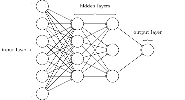
In between are several hidden layers. In these layers, each neuron uses the outputs of the layer before as inputs. The outputs, in turn, are used as the inputs for the next layer. This is how neurons are connected.

So, what’s the advantage of this structure?

Networks In Practice

Neural networks allow us to solve problems that other structures can’t. One well-known example is identifying digits.

Suppose we want our neural network to accept images of numbers and to “read” the number. These digits are handwritten, so they vary in size, location, shape, etc.

We could start by considering what our input layer might be. Since the image is comprized of pixels, we can imagine a layer of neurons that each represent a pixel. The shade of the pixel can serve as the value of each neuron.

In the first hidden layer, each neuron will look for an assigned mark. Certain groups of pixels could indicate the presence of the component. The neurons which detect the mark will return a value closer to $1$.

The remaining hidden layers will attempt to “assemble” the number. These layers will compile clusters of marks in bigger marks and curbes and, eventually, into loops and lines.

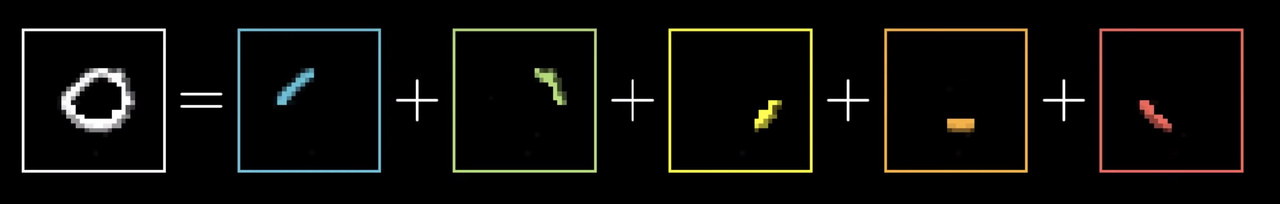
Finally, the output layer would take these biggests parts—loops and lines—and return the predicted number. For example, an upper and lower circle could indicate an eight.

This is what the neural network would look like in action:

The XOR Problem

Today, we will implement a solution to the XOR Problem. The XOR Problem was one of the first challenges for neural networks. The challenge was to design an algorithm that could correctly classify predict the outcome of a XOR gate.

The XOR gate is simple. The gate accepts two Boolean inputs, A and B, and only returns true if A is not B.

But, simple classifiers won’t work here. For example, if we try to use linear regression, we quickly find out that no line can split the data.

We’re going to resolve this with neural networks. We want a model that can “bend” the space so that the two points can be separated.

How does the neural network do this?

The key is to design an activation function, which enables us to escape linearity.

Prerequisites

Linear Algebra

Say we’re given two matrices, $A$ and $B$, with dimensions $m\times n$ and $p\times q$, respectively.

To multiply them together, we multiply each row in $A$ by each column in $B$, multiplying the corresponding entries and summing them. For this to work, there need to be the same number of rows in $A$ as columns in $B$—$n$ must equal $p$—so that each entry has something with which to multiply.

The sum of the products of multiplying row $x$ from $A$ with column $y$ from $B$ is entered into $C_{x, y}$.

<img src="https://i1.wp.com/www.javatechblog.com/wp-content/uploads/2016/06/matrix-multiplication.jpg?resize=583%2C565" height=300>

Calculus

As we said in an earlier lecture, gradient descent is the algorithm we use to minimize the cost function, which is a measure of how well our regression function fits our data.

A derivative is the slope of a function with respect to a variable that changes. Functions, however, can be of multiple variables (e.g. $f(x,y)=x^2y$). In a partial derivative, we hold all but one of the variables constant.

$\frac{\partial f}{\partial x}$ would represent the partial derivative of $f$ with respect to $x$, while $\frac{\partial f}{\partial y}$ would show the partial derivative of $f$ with respect to $y$.

To find our gradient at each point, we store the partial derivatives of each variable in the function.

A composition function can be represented by $f(g(x))$, where $g$ can also be a composed function. In order to calculate $f$, we must first calculate $g$. Neural networks compose all the hidden layers to create one final function, where to calculate the output of each layer we first need the output of the previous one.

To take the derivative of a composite function, we use the chain rule. The chain rule says that, if $f(x) = f(g(x))$, its derivative would be $\frac{d}{dx}f(g(x))\cdot \frac{d}{dx}g(x)$. In other words, to calculate the derivative of a composite function, we find the product of the derivative at each step.

Python

This time in python, we will be using a module that you will find yourself using very often in the world of machine learning in python: Numpy.

import numpy as np

class Class_Name():
    def __init__(self, var_3):
        self.variable_3 = var_3
        
    ### There is now a new variable called var
        
    def my_function(self, var_1):
        return var_1


    ### EXAMPLE:
    def __init__(self, layer1, layer2):
        self.layer1 = layer1
        self.layer2 = layer2
        
    def sigmoid(self, x):
        return 1 / (1 + exp(-x))

    def sigmoid_derivative(self, x):
        return x * (1 - x)

Getting Started with Neural Networks

Each neuron in a multilayer perceptron has both a weight and a bias. You can think of this weight and bias as a knob for changing your function.

All neurons in the hidden and output layer are initailized with random weights and biases. Note: in most cases, the input layer will also have weights and biases; however, for the sake of demonstration, we will disregard this for the time being.

Let’s mathematically define our hidden layer, starting with just the $a_4$ node. First we will take all the inputs and multiply them by their respective weights. Each synapse—line connection—takes the input and multiplies it by some weight. Each input has its own weight. We should get something similar to:

$$a_4 = x_1 \cdot w_{41} + x_2 \cdot w_{42} + x_3 \cdot w_{43}$$

To denote the weights, we use $w_{\text{hidden_layer}}{\text{input_node}}$. For the sake of demonstration and optimization, we will not need to use a bias. For each following node in the hidden layer, it will take the same inputs, but use different weights.

$$a_5 = x_1 \cdot w_{51} + x_2 \cdot w_{52} + x_3 \cdot w_{53}$$ $$a_6 = x_1 \cdot w_{61} + x_2 \cdot w_{62} + x_3 \cdot w_{63}$$ $$a_7 = x_1 \cdot w_{71} + x_2 \cdot w_{72} + x_3 \cdot w_{73}$$

Based on what we learned earlier, let’s try to express this in terms of linear algebra. First, let’s use a vector to describe all of our inputs:

$$x=\begin{bmatrix} x_1 \\ x_2 \\ x_3 \end{bmatrix}$$

We only ever have three inputs. However, for each node in our hidden layer we will be multiply these nodes, each by their own weight.

$$W^T = \begin{bmatrix} w_{41} \ w_{42} \ w_{43} \\ w_{51} \ w_{52} \ w_{53} \\ w_{61} \ w_{62} \ w_{63} \\ w_{71} \ w_{72} \ w_{73} \end{bmatrix}$$

By simply performing matrix multiplication we get a vector for our entire hidden layer:

$$a = x \cdot W^T_1$$

A more visual view of the calculations the matrix will perform:

$$a = \begin{bmatrix} x_1 \cdot w_{41} + x_2 \cdot w_{42} + x_3 \cdot w_{43} \\ x_1 \cdot w_{51} + x_2 \cdot w_{52} + x_3 \cdot w_{53} \\ x_1 \cdot w_{61} + x_2 \cdot w_{62} + x_3 \cdot w_{63} \\ x_1 \cdot w_{71} + x_2 \cdot w_{72} + x_3 \cdot w_{73} \end{bmatrix}$$

Now we want to get the the output, the y values. To do this, we will use matrix multiplication again. Imagine this to be exactly the same as the input to hidden layer part. This time we’re going from $a$ to $y$, or from $4$ to $2$.

$$y = a \cdot W^T_2$$

So if we want to create a single function for our entire neural network, it is simple:

$$y = (x \cdot W^T_1)\cdot W^T_2$$

On a fundamental level, multilayer perceptrons—a type of neural network—are just giant composite functions. If we had more layers, we would just be multiplying by more weights. All of these weights are the knobs and dials of our function that allow us to customize our function to fit the data.

Take some time to play around with the tensorflow playground to get a better idea of how these knobs interact with one another.

So now we have our predictions for our final answers. How do we go about editing these weights? Let’s start by checking our predictions. To do this, we will use something called a cost function.

Cost Function

This table might be seem pretty complex, but we’re only interested in the first cost function. If you remember back to our linear algebra lecture this is a very similar as we are trying to calculate how well our model is doing at predicting values.

Now that we have our cost function, we can understand both how our model is doing, and how to make our model better.

Backpropagation

The way we actually want to go back and edit our weights is with a technique known as backpropagation. For today we will go over a very basic example, just to introduce the concept.

We use this model:

Now, we define a cost function that measures how far our model is from our desired output:

Remember Gradient Descent? We could the use slope or rate of change of the function to find the minimum of the function.

The rule looks like this:

$$w_{t+1} = w_t -r \frac{\partial C}{\partial w}$$

We nudge the weights by a multiple of the gradient.

Since $C(a) = (a-y)^2$ is defined in terms of a (y is constant), we can find how $C(a)$ changes relative to $a$ with ease.

The rate of change is: $\frac{\partial C}{\partial a}=2(a-y)$

But, this is really not useful because the only value we could change is $w$, the weight, not the activation.

What we really want is $\frac{\partial C}{\partial w}$, or how the weight affects the cost function.

Enter the chain rule. We could mulitply the rates, as if the fractions cancelled out.

$$\frac{\partial C}{\partial w}=\frac{\partial C}{\partial a}\frac{\partial a}{\partial w}$$

The last derivative, $\frac{\partial a}{\partial w}$, is quite simple because it is a linear relationship: $a = i \cdot w$.

So, the rate of change is just $\frac{\partial a}{\partial w} = i$

The final gradient is $\frac{\partial C}{\partial w}= i \cdot 2 (a - y)$; written in terms of $i$, it would be $\frac{\partial C}{\partial w}= i \cdot 2 (i \cdot w - y)$.

Now, try plugging in the numbers, $i=1.5$ and $y=0.5$. You should get something like this:

$\frac{\partial C}{\partial w}=4.5w-1.5$ $$

Lets get back to our original algorithm, Gradient Descent:

$$w_{t+1} = w_t -r \frac{\partial C}{\partial w}$$

We iteratively update our weights according to the slope. Here is an example:

Your Turn

Let’s start off by just working with basic perceptrons. Start by going to tensorflow playground.

Once you feel like you’ve exhausted your combinations, or are simply bored, let’s try implementing your first neural network. We’ve already created a class system for you that you can use in Python to actually implement a neural network. Start by creating a colab by going to google colab and creating a new google colab in Python3.

Feel free to copy the code below (this is code you do not have to feel like you completely understand):

from numpy import exp, array, random, dot


class NeuronLayer():
    def __init__(self, number_of_neurons, number_of_inputs_per_neuron):
        self.synaptic_weights = 2 * random.random((number_of_inputs_per_neuron, number_of_neurons)) - 1


class NeuralNetwork():
    # Create the first 2 layers
    def __init__(self, layer1, layer2):
        self.layer1 = layer1
        self.layer2 = layer2

    # Used for forward propagation
    def sigmoid(self, x):
        return 1 / (1 + exp(-x))

    # Used for backpropagation
    def sigmoid_derivative(self, x):
        return x * (1 - x)

    # Training and backprop
    def train(self, training_set_inputs, training_set_outputs, number_of_training_iterations):
        for iteration in range(number_of_training_iterations):
            output_from_layer_1, output_from_layer_2 = self.test(training_set_inputs)
            
            # Backprop
            layer2_error = training_set_outputs - output_from_layer_2
            layer2_delta = layer2_error * self.sigmoid_derivative(output_from_layer_2)
            
            # Backprop
            layer1_error = layer2_delta.dot(self.layer2.synaptic_weights.T)
            layer1_delta = layer1_error * self.sigmoid_derivative(output_from_layer_1)

            # Fine Tuning
            layer1_adjustment = training_set_inputs.T.dot(layer1_delta)
            layer2_adjustment = output_from_layer_1.T.dot(layer2_delta)

            # Edit weights
            self.layer1.synaptic_weights += layer1_adjustment
            self.layer2.synaptic_weights += layer2_adjustment

    def test(self, inputs):
        output_from_layer1 = self.sigmoid(dot(inputs, self.layer1.synaptic_weights))
        output_from_layer2 = self.sigmoid(dot(output_from_layer1, self.layer2.synaptic_weights))
        return output_from_layer1, output_from_layer2

This class can only generate three layer neural networks with one hidden layer. Let’s start by creating our layers:

input_layer_size = 2
hidden_layer_size = 3
output_layer_size = 1

layer1 = NeuronLayer(hidden_layer_size, input_layer_size)
layer2 = NeuronLayer(output_layer_size, hidden_layer_size)

# initialize my neural network
neural_network = NeuralNetwork(layer1, layer2)

Let’s now add our data:

# features
training_set_inputs = array([[0, 0], [0, 1], [1, 0], [1, 1]])

# labels
training_set_outputs = array([[0, 1, 1, 0]]).T

Train our neural network:

iterations = 10000
# training
neural_network.train(training_set_inputs, training_set_outputs, iterations)

Next, let’s test our neural network:

print("Our results: ")
print("0, 0")
hidden_state, output = neural_network.test(array([0, 0]))
print("Guessed output: "+str(round(float(output)))+ " | Percent Certainty: "+str(round(1-output[0], 2)))
print("___")
print("0, 1")
hidden_state, output = neural_network.test(array([0, 1]))
print("Guessed output: "+str(round(float(output)))+ " | Percent Certainty: "+str(round(output[0], 2)))
print("___")
print("1, 0")
hidden_state, output = neural_network.test(array([1, 0]))
print("Guessed output: "+str(round(float(output)))+ " | Percent Certainty: "+str(round(output[0], 2)))
print("___")
print("1, 1")
hidden_state, output = neural_network.test(array([1, 1]))
print("Guessed output: "+str(round(float(output)))+ " | Percent Certainty: "+str(round(1-output[0], 2)))

Lastly, let’s generate a 3D graph of our values (this is code you do not have to feel like you completely understand):

x_arr = []
y_arr = []
z_arr = []
count = 0
for each in range(0, 10):
  count_two = 0
  y = 0+count/10
  for eachT in range(0, 10):
    x = 0 + count_two/10
    hidden_state, output = neural_network.test(array([x, y]))
    x_arr.append(x)
    y_arr.append(y)
    z_arr.append(output.tolist()[0])

    count_two += 1
  count += 1

from mpl_toolkits import mplot3d
import matplotlib.pyplot as plt
import numpy as np

x = np.reshape(np.asarray(x_arr), (10, 10))
y = np.reshape(np.asarray(y_arr), (10, 10))
z = np.reshape(np.asarray(z_arr), (10, 10))

print("\n")
fig = plt.figure()
ax = fig.add_subplot(111, projection='3d')

ax.plot_surface(x, y, z, rstride=1, cstride=1, cmap='viridis', edgecolor='none')

ax.set_xlabel('X Label')
ax.set_ylabel('Y Label')
ax.set_zlabel('Z Label')

plt.show()


fig = plt.figure()
ax = fig.add_subplot(111, projection='3d')
ax.plot_wireframe(x, y, z, rstride=1, cstride=1)

ax.set_xlabel('X Label')
ax.set_ylabel('Y Label')
ax.set_zlabel('Z Label')

plt.show()

Our solution to XOR and a demonstration of XOR implemented in TensorFlow: click here.

Disclaimer: The TensorFlow implementation was written by Martin Thoma