Background

Some philosophical stuff

Artificial intelligence and machine learning are at the forefront of computer science, but what do they mean?

Artificial intelligence is defined as “the science and engineering of making intelligent machines” by John McCarthy, one of Gautom’s idols. It can also be thought of as the capability of a machine to imitate intelligent human behavior. AI encompasses many fields, including machine learning and deep learning.

And machine learning?

Machine learning programs alter themselves. They learn dynamically—without human intervention—from the data. As another one of Gautom’s favorite people, Arthur Samuel, said, machine learning is the “field of study that gives computers the ability to learn without being explicitly programmed.” This is where the cool stuff happens. In a machine learning algorithm, the goal is to minimize cost (error), which is what we’ll be learning about today.

Prerequisites

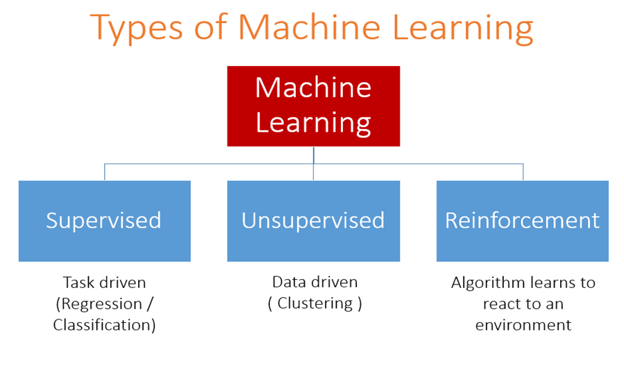
By now, you should be familiar with everything covered in the AI Begins lecture. You must know the different types of machine learning and have minimal experience in python as well as the linear regression covered in that lecture.

Model Terminology

For our supervised learning models,

• $x_i$ will denote an item in our list of inputs, or features
• $y_i$ will denote an item in our list of output, or labels
• $m$ will be the amount of training points (the amount of $i$s)
  • Note that $i$ is simply an index (think of python lists)
• A pair $(x_i, y_i)$ will be a training example
• $X$ and $Y$ will represent the space of output/input values
  • For this example, $Y=X=\mathbb{R}$

Can you spot each of these terms in the context of this graph?

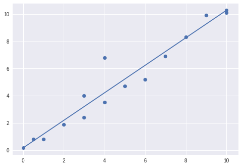
For our supervised learning problems, our goal will be to use our training points (of features and labels) to make a hypothesis, or prediction. This hypothesis will be called $h(x)$:

$$h(x) = w_0x + w_1$$

Look familiar? In our linear regression model from last time, this prediction function is commonly known as the line of best fit.

If our label is a continuous range, we would call this a regression problem; if it is a series of concrete labels, (C-section vs No C-section) we call our problem a classification problem.

Evaluating our Hypothesis

To get the best possible $h(x)$, we must determine a way to evaluate it—to determine if we’ve made an accurate prediction or a shitty one. This is called our cost function. There are many different ways to evaluate this function, but the one we’ll be using is mean squared error (MSE), which follows this equation:

$$J(w_0, w_1)=\frac{1}{2m}\sum_{i=1}^m{(h_w(x_i)-y_i)^2}$$

Other cost functions include:

• Cross-entropy cost
• Exponential cost
• Hellinger distance
• Kullback-Leibler divergence
• Generalized Kullback Leibler divergence
• Itakura-saito distance

Our goal is to minimize the cost function, no matter which we choose.

Can you think of what would happen if instead of squaring our difference (MSE), we cubed it? What problems would we face, and how could we resolve them?

Visualizing the Cost Function

One Parameter

Imagine our hypothesis is defined as:

$$h(w_0) = w_0x$$

and our training points are plotted as such:

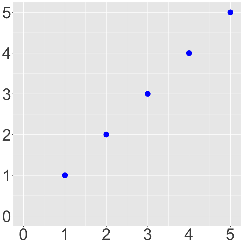
For this example, our prediction is fairly obvious ($w=1$); if we change $w$ to $\frac{1}{2}$ or $2$, our cost function will obviously increase, since the prediction function isn’t fitting our data as well as it could.

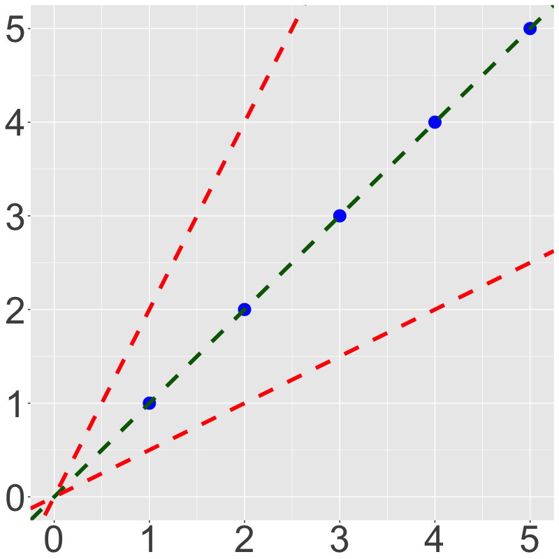
By plotting $w$ against cost, we can see how diverging from $w=1$ will make our model less effective.

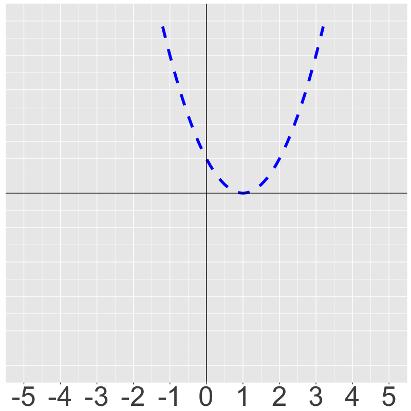
Training our model means finding the basin—the absolute minimum—of this cost function.

Two variable

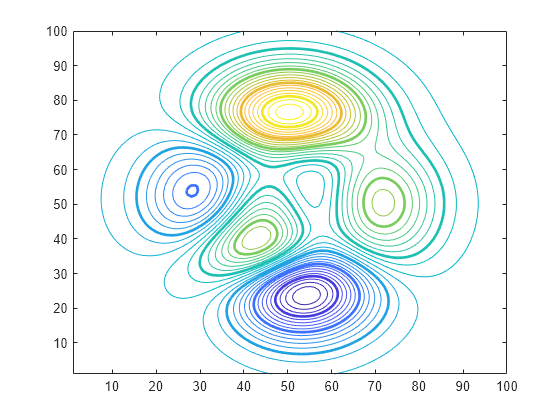
Now, let’s say our prediction will take two variables:

$$h(w_1,w_2)=w_1x+w_2$$

Visualizing our cost function will now require another dimension. This can be visualized in two ways: a 3d graph, or a contour plot:

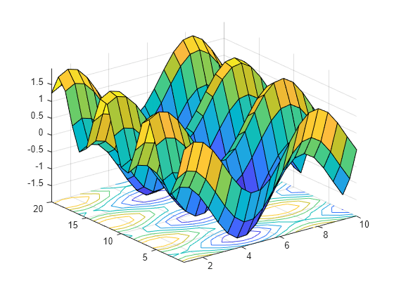
Again, our training mission will be to find the lowest point on this graph, minimizing the cost function. Adding another variable would be pretty much impossible to visualize—unless you went for a 3d contour plot.

Gradient Descent

For higher-parameter problems, we need gradient descent. Gradient descent is a method of finding local minimums in functions by making tiny changes to the weights in $h$, our hypothesis.

The formula

To start off, the gradient descent algorithm follows this function, where $\alpha$ is the learning rate:

$$w_j:=w_j-\alpha\frac{\delta}{\delta w_j}J(w_0,w_1) \\ b=a-\gamma\nabla f(a)$$

The ball analogy

Gradient descent can be thought of through a simple ball drop analogy. Consider the following diagram:

Here, as the graph gets a better prediction, the “ball” showing the current parameter values gets lower into the basin of costs function.

This works because gradient descent gets the slope at your current point and moves a step in that direction. The steeper your slope, the farther the ball will move. In this case, the learning rate is a coefficient on your step (the size of your step).

Gradient Descent Considerations

Simultaneous update

Gradient descent, to work properly, uses a simultaneous update, so you must update the parameters at the same time or with the same parameter values. Refer to the following diagram:

$$temp_0 := w_0-\alpha\frac{\delta}{\delta w_0}J(w_0,w_1) \\ temp_1 := w_1-\alpha\frac{\delta}{\delta w_1}J(w_0,w_1) \\ w_0:=temp_0 \\ w_1:=temp_1$$

If we didn’t do it this way, what would our gradient descent look like? Would it work?

Local minima

There’s a fairly major difference between the requirements of machine learning and gradient descent’s function: machine learning calls for a global minimum, while Gradient descent finds local minima. Imagine performing gradient descent on a function like this one:

Yeah, that would suck. It would likely do something like this:

You’ll learn how to overcome this later.

Why simultaneous gradient descent won’t always work

This is an example of a vector field that isn’t conservative. (A conservative vector field is a slope field that represents the gradient of some function.) While there is equilibrium at $(0,0)$, simultaneous gradient descent will never solve it. Don’t worry, this reaches a level of abstraction greater than we’ll reach, so you won’t encounter something like this.

Overfitting and underfitting

Goldilocksing your data

Overfitting and underfitting your data are two of the hardest obstacles of machine learning. All beginners struggle with this obstacle; it touches every realm of machine learning and data science.

Consider this scenario:

You make an algorithm that predicts whether or not a patient will need a C-Section based on age, body weight, diet, and hair color.

You design your model, and train it.

Woah! You’ve taught your model to fit your training set, and you have 99% accuracy. You’re ready to make some predictions for the hospital you work in (with the goal of cutting costs).

You’re all hyped up to get a big, fat, chunky raise, but when you make your real predictions, you only get 50% accuracy. You now live under a bridge and eat roadkill.

This will happen when our model doesn’t generalize well in the translation between training points and actual predictions. This diagram shows how we can overfit, underfit, and hit that Goldilocks sweet spot.

This actually doesn’t only happen in data science. It happens everywhere. This video is particularly good at pointing out this phenomenon.

Signal and noise

That’s also the name of a very good book—The Signal and the Noise—about why predictions fail by Nate Silver, Prayag’s idol.

In predictive modeling, there are two traits to a dataset:

• Signal: The general pattern or direction of the data—what is important
• Noise: Irrelevant information and randomness in our dataset

What would our signal be for Age vs Height? Noise?

In machine learning, you want to properly determine your signal so as not to underfit your data, while ignoring noise so as not to overfit it. Noise will always exist, so it’s important to learn how to deal with it.

Avoiding overfitting

The best way to avoid overfitting and underfitting is keeping two datasets separate. If your training set performs considerably better than your test set, you are likely overfitting.

The other way to avoid overfitting is using the Occam’s razor test. If you have two models with comparable performance, using the simpler one is normally the best idea. This means sometimes starting with simpler models—like linear regression!

Sometimes, simply removing extraneous features helps against overfitting.

Closing up

Over the last two lectures, we’ve discussed a few main ideas. If you have any questions about these, please ask:

• The different types of machine learning
• What linear regression is and how to calculate it
• The goal of supervised learning
• The cost function
• Gradient descent and its intricacies
• How to avoid over/underfitting

Again feel free to ask questions, either now or over email. See you all next week!