AI Begins

Popular Testimonials

The development of full artificial intelligence could spell the end of the human race … it would take off on its own, and re-design itself at an ever increasing rate. Humans, who are limited by slow biological evolution, couldn’t compete, and would be superseded.

Stephen Hawking, 2014

A more interesting quote:

Artificial intelligence is the future, not only for Russian, but for all of humankind. It comes with colossal opportunities, but also threats that are difficult to predict. Whoever becomes the leader in this sphere will become the ruler of the world.

Vladimir Putin, 2017

What is AI?

Background

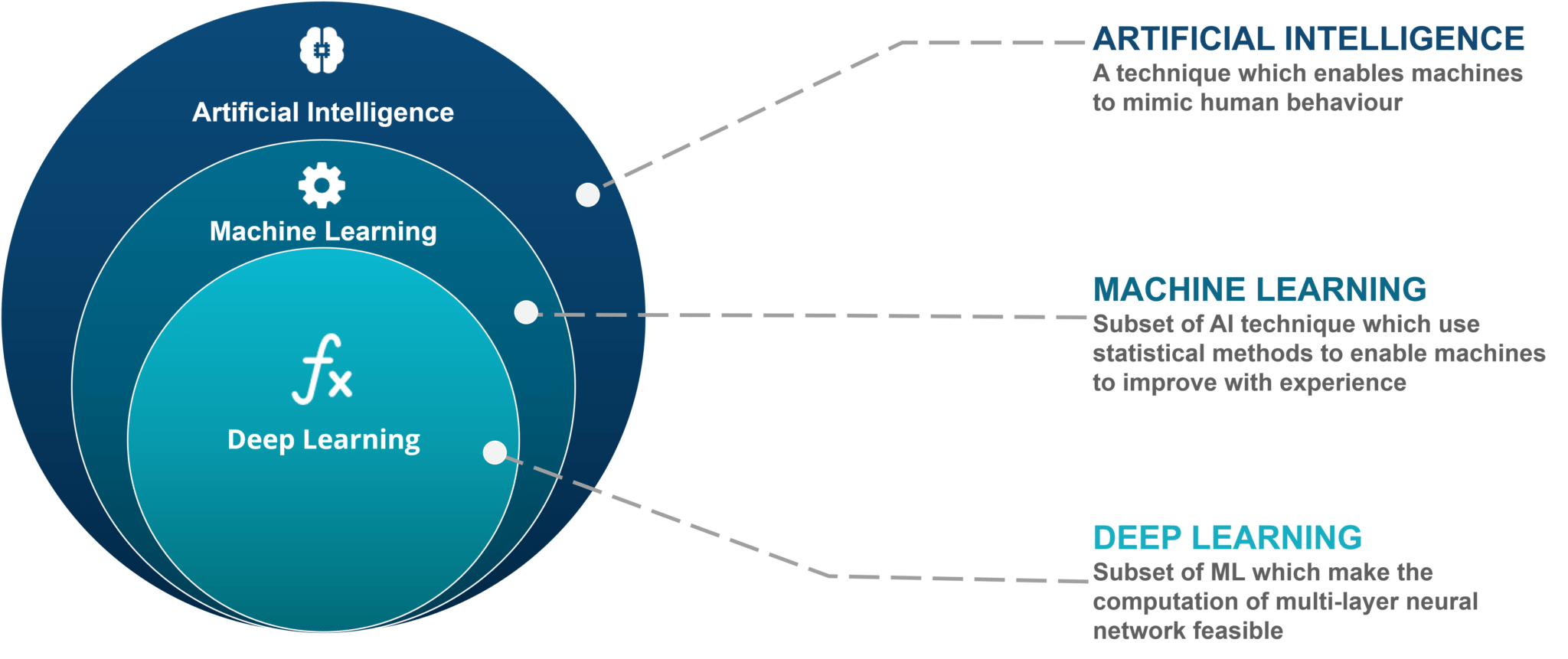
Artificial Intelligence: A machine demonstrating intelligence.

Having machines that think has long since been a dream dating back to the Ancient Greeks. The idea really saw the light of day again when programmable machines were created.

History & Real World Examples

Turing Test A test of a machine’s ability to exhibit intelligent behavior equivalent to, or indistinguishable from, that of a human.

Hard Coding Knowledge At the beginning of the 1960s, many new projects took on the task of hard coding knowledge and logic. One of the most successful was the Cyc project. Starting in 1984, it contains 30 years of knowledge. There have been a few open source and beta releases in the early 2000s, but today it is considered a “catastrophic failure.”

This suggested a need for AI to have the ability to extract patterns.

Chess Initially, there were two preferred methods: the brute force algorithm and the strategic AI. Which do you think would be preferred?

The Brute Force Method.

In the early 1960s, computing power was limited; by the early 1970s, however, computing power was strong enough to effectively use Brute Force. IBM’s Deep Blue uses the Brute Force method.

AI Winter In the mid 1970s, the government stopped funding AI during the Cold War. This was the result of two reports—the ALPAC report and the Lighthill report—which claimed that machine translation was hopeless.

Logistic Regression Although linear regression has been around since the 1800s, logistic regression was only invented in the 1950s. Following this, more intuitive techniques appeared, one of the most popular being logistic regression. This technique was used in the 1990s to accurately determine whether or not a women needed a Caesarean Section.

Modern AI AI has slowly found its way everywhere and is now here to stay. You can find its implementation in emails, social media, driving, advertising, and many other fields.

Terminology

Labels: The labels for a given dataset. Think of it as the $y$ in a Cartesian function.

Features: The features for a given dataset. Think of it as the $x$ in a Cartesian function.

Models: As per Amazon’s definition, “model” refers to the model artifact that is created by the training process.

Training: Incrementally improving a given algorithm.

Regression Model: The output is a continuous value.

Classification Model: The output is a label or a class.

Supervised Learning: You have labels and you’re training a model.

Unsupervised Learning: You don’t have labels and you’re trying to find a relationship in the data.

Machine Learning vs. Deep Learning

Prerequisites

Data Formatting

Variables: Values that can change and pass information onto a program.

Arrays: Used to store series of values and can have any number of dimensions. How many dimensions would an RGB picture have?

Index: The location of an element in a given array. In Python (and in many other languages), the first element in an array is 0.

Language & Environment

The main language that we will be using is Python—specificially version 3.6. Head over to Google Colab. When there, create a new Python 3 journal.

Python Cheat Sheet

#This is a comment, indicated by the "#"
import module_name #import a package

variable_name = value #set a new variable
#dog_type =  "Poodle"
#dog_numb = 50
#dog_list = ["Poodle 1", "Poodle 2", "Poodle 3"]

print("Output to Console") #output to the console

example_array = ["a", "b", "c", "d"] #create an array, wherein example_array[2] would be "c"

twoD_array = [[1,2], [2,3], [3,4], [4,5]] #create a 2D array. Think of this as a table

var = var + 1
#this is the same as
var += 1

for each in items:
    print(each)

def function(variable):
    operation += variable
    return operation

Using Google Colab

First, install the packages needed for your project, starting by creating a new code cell. In that code cell, type !pip install plus whatever other packages you need.

Linear Regression Potpourri

One Leap: Normal Method

Start off with the generic formula for a line:

$$y = w_0 + w_1x$$

Our goal is to find $w_0$ and $w_1$. These are the parameters of the equation, or—in ML jargon—the weights.

If we start putting more $x$’s:

$$y = w_0 + w_1x_1 + w_2x_2 + ... + w_nx_n$$

Now, we try to find all the $w$’s. We can express this more concisely using the dot product:

$$y_m = X_m \cdotp w$$

Where $X_m$ is the inputs for one example, $y_m$ is the output for the that example.

$X_m = \begin{bmatrix} ​ 1 \space x_{1} \space x_{2} \dots x_{n} ​ \end{bmatrix}$ $w = \begin{bmatrix} ​ w_{0} \\ ​ w_{1} \\ ​ \vdots \\ ​ w_{m} ​ \end{bmatrix}$ We next try to find the vector, $w$. If we stack multiple examples together:

$$y = Xw$$

Where

$X = \begin{bmatrix} ​ X_{1} \\ ​ X_{2} \\ ​ \vdots \\ ​ X_{m} ​ \end{bmatrix}$ and

$$y = \begin{bmatrix} ​ y_{1} \\ ​ y_{2} \\ ​ \vdots \\ ​ y_{m} ​ \end{bmatrix}$$

There are several advantages to using matrices:

• It’s easy to write down as an equation with simple multiplication
• There are good linear algebra libraries to speed up matrix multiplication

Expressing it as a matrix expression, we can unleash the full power of inverses. However, most of the time, the equation cannot just be solved with a simple inverse.

This occurs because all the points of linear regression don’t fit on the line, but are actually only close to it.

Then some magic later, we arrive at:

$$w = (X^TX)^{-1}X^Ty$$

What’s really happening here is that we’re projecting $y$ and $Xw$ into a subspace through $X^T$.

$$X^TXw = X^Ty$$

Then, we invert by $X^TX$ to isolate $w$, the weights, which is exactly what we want.

This is the code in python:

w = np.dot(np.linalg.inv(np.dot(X.T, X)), np.dot(X.T, y)

Notebook link

Practical Application

Given the equation of a line: $y=mx+b$

And then given the equation:

$$m = \frac{\sum\limits_{}(x_i-\bar{x})(y_i-\bar{y})}{\sum\limits_{}(x_i-\bar{x})^2}$$

For $b$, sub back in $\bar{y}$, $\bar{x}$, and $m$.

$$b = \bar{y}-m\bar{x}$$

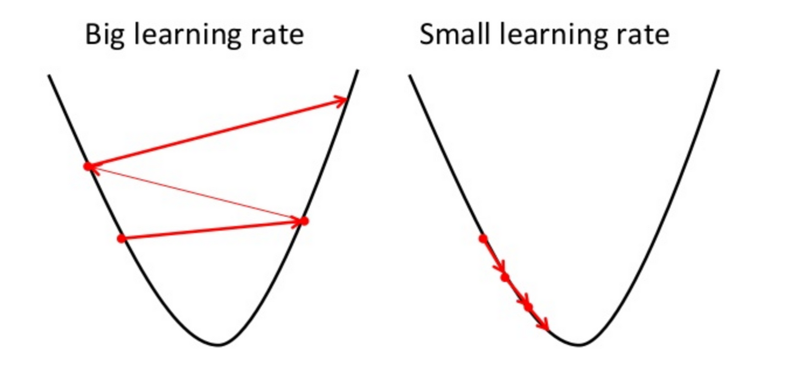
Black Box: Gradient Descent

Start off with the generic formula for a line:

$$h_\theta(x) = \theta_0+\theta_1x$$

This is equivalent to $h(x) = mx + b$, but research papers usually use the $\theta$ (theta) notation.

Using generic values of $\theta_0$ and $\theta_1$:

$$\theta_0, \theta_1 = 1$$

And repeat the following algorithm until convergence:

$$\theta_0 = \theta_0 - \alpha\cdot\frac{1}{m}\sum_{i=1}^m(h_\theta(x^i)-y^i)$$ $$\theta_1 = \theta_1 - \alpha\cdot\frac{1}{m}\sum_{i=1}^m(h_\theta(x^i)-y^i)\cdot x^i$$

Linear Regression Implementation

The goal of this task is to both use Google Colab and to practice implementing a formula in Python. We’ll start with a dataset of $x$ and $y$ values and then graphing them. The library we will be using for graphing will be matplotlib. If you are getting an import error, run !pip install matplotlib.

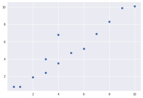
Use the following code to display a scatter plot:

import matplotlib.pyplot as plt

x = [0.5, 1, 2, 3, 4, 5, 6, 7, 8, 9, 10, 4, 3]
y = [0.8, 0.8, 1.9, 2.4, 3.5, 4.7, 5.2, 6.9, 8.3, 9.9, 10.1, 6.8, 4]

points = [x, y]
plt.scatter(x, y);

In Google Colab, start by going to File > New Python 3 notebook. From there, add a new Code Cell, paste in the above code, and run it by clicking on the play button. You should see something similar to this:

From there, we’ll add our line of best fit based on the equation.

Practical Application Let’s start by breaking down the equation for slope:

$$m = \frac{\sum\limits_{}(x_i-\bar{x})(y_i-\bar{y})}{\sum\limits_{}(x_i-\bar{x})^2}$$

The $\sum$ symbol refers to a sum. In this particular equation, $\bar{x}$ and $\bar{y}$ refer to the mean of all $x$ points and $y$ points.

Now, we calculate $\bar{x}$ and $\bar{y}$ (the means).

x_sum = 0
y_sum = 0

for x_p in x: #call each element in list x "x_p"
  x_sum = x_sum + x_p
  
for y_p in y:
  y_sum = y_sum + y_p
  
numb_elem = len(x)

#x hat is the same as mean of x
x_mean = x_sum/numb_elem
#y hat is the same as mean of y
y_mean = y_sum/numb_elem

Since the length of x and y are the same, they can both be used for the length of the list. From there, let’s calculate the sums in the numerator and in the denominator.

#top sum
top_sum = 0

count = 0
for x_val in x:
  x_p = x_val
  y_p = y[count]
  count += 1
  
  x_minux_x_hat = x_p - x_mean
  y_minux_y_hat = y_p - y_mean
  
  top = x_minux_x_hat * y_minux_y_hat
  # using += is the same as the var plus itself and some value
  # var = var + 1
  # is the same as
  # var += 1
  top_sum += top

#bottom sum
bottom_sum = 0
for x_val in x:
  x_minux_x_hat = x_val - x_mean
  bottom = x_minux_x_hat * x_minux_x_hat
  # using += is the same as the var plus itself and some value
  # var = var + 1
  # is the same as
  # var += 1
  bottom_sum += bottom

Now that we have both the top sum and the bottom sum, we can find m by simply dividing the top sum by the bottom sum:

m = top_sum/bottom_sum

Now, all we have to do is find $b$ to complete our $y=mx+b$ equation. We will simply use basic algebra. First, move $mx$ to the other side of the equation to get $b=y-mx$. We need an $x$ and a $y$ to find $b$. What can we use? The original mean point! This gives us:

$$b = \bar{y}-m\bar{x}$$

Which translates to:

b = y_mean - m * x_mean

Finish up by adding the following code:

print("Our final equation is: y = " + str(round(m, 2)) + "x + " + str(round(b, 2)))

def mx_formula(x):
  return m*x + b

import matplotlib.pyplot as plt
import matplotlib.lines as mlines

x1, y1 = [0, 10], [b, mx_formula(10)]
plt.plot(x1, y1, marker = 'o')
plt.scatter(x, y)

This will simply convert your final equation into a line on a scatter plot. Hit run and you should see something similar to:

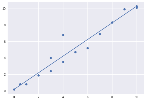
Congrats! You’ve now completed linear regression using least squares from scratch. Click here to view the entire journal. Next week, we’ll move on to more complicated techniques and dig deeper into Gradient Descent.