
Introduction
We’ve been using cleaned and well-structured data from, for example, the MNIST database to practice and better understand machine learning. But data (plural) don’t often come cleaned and ready-to-use; instead, we usually have to compile multiple databases, remove rows, reformat columns, change the database structure—the list goes on.
Purpose
R is the best and most used language for data manipulating and visualizing and for statistical modeling, and it’s even an emerging competitor in the machine learning world. It’s primarily used by academics and data scientists, though with some up-and-coming packages and features—namely, Shiny and R Markdown—R is pushing into the business world.
R vs. Python
R and Python were built by different people for different people. R was programmed by statisticians sick of its lowkey disgusting predecessor, S, while computer scientists created Python as a general, easy-to-read programming language.
R works best for manipulation on big data (which are often hosted externally; because of this, R has good tools for SQL integration), while Python is faster for smaller tasks. R also has more built-in statistical modeling functions (and is used more than Python for such projects), but Python is easier to read for less adept programmers when writing a new model.
Code in R is a lot less structured that in Python, which can lead to some messy files. Follow the Google R Style Guide so you don’t drive people crazy.
Setup
RStudio
Pretty much every R user codes in RStudio. It’s easy to see why—the default orientation splits the screen into four, with easy access to an editor, where you can write scripts and view databases; the console, which accesses the same environments as the code you’ve run in that session; a list of variables and what they represent; and a viewer, which is generally used for plots, files, and the help menu. RStudio also integrates nicely with GitHub.

Download R here and RStudio here. To edit R code online, use rdrr.
Useful packages
Once you finish up the installation, it’ll be time to download some good packages. Navigate to Tools⟶Install Packages... and enter, separated by commas:
tidyverse, which will downloadggplot2, for data visualizationdplyr, for data manipulationtidyr, for data tidyingreadr, for data importpurrr, for functional programmingtibble, for tibbles, a modern re-imagining of data framesstringr, for stringsforcats, for factors
rvest, for scraping websites (maybe another lecture)devtools, for easily downloading random packages from GitHubggthemes, for more plot themesleaflet, for making maps
Those are just some good ones to start with; as you do more diverse things with R, you’ll find new packages to download—and you might just write one of your own.
Load packages with require(package_name) or library(package_name). require will return a warning, not an error, while library will terminate the program. There’s no real difference in speed or anything else, so it doesn’t really matter which one you use.
General
Below are some helpful suggestions about RStudio and R in general:
- Use the projects feature—it’ll be easier to open a bunch of files at once
- Open your dataframes in the viewer by clicking on them in the variable panel
- When you first open/create your programs, make sure you click
Session⟶Set Working Directory⟶To Source File Location - Turn on “Source on Save”; this lets you run a file by simply saving it
- You’ll often see people use variable names like
fooandbar—these are helpful for Stack Overflow responses and don’t actually mean anything- Many questions also reference the
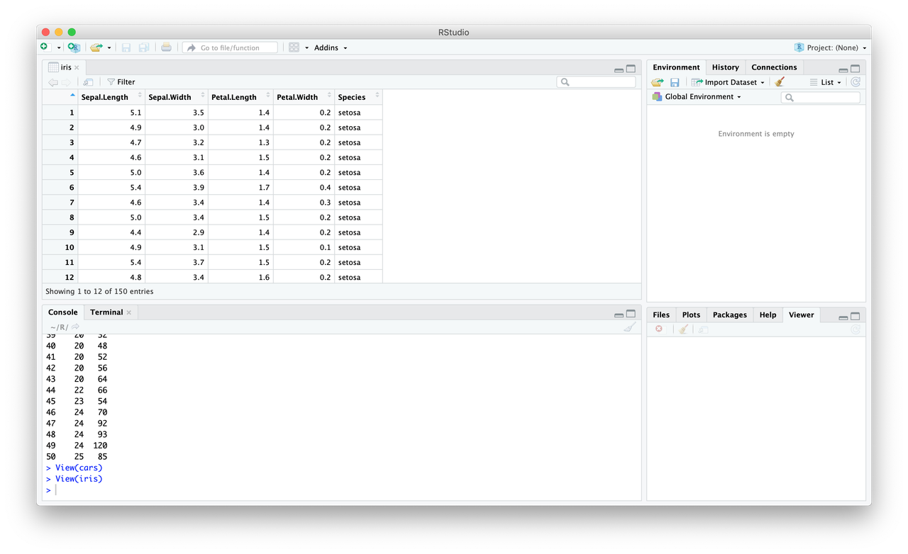
carsdatabase, which is one of many that are pre-installed in R
- Many questions also reference the
- Missing data are represented with
NA - Non-numbers (e.g. $\frac{0}{0}$, $\frac{\infty}{\infty}$, etc.) are represented with
NaN dfis often used as a half-assed variable name for a “dataframe,” the main way to store a table of data in R
And here are some useful code bits and what they do:
- Comment with
# - Indentation doesn’t matter
- No need for semicolons
- Figure out what a function does by simply typing
?function_namein the console. Note the lack of parenthesis - If you’re writing code with multiple packages where some functions may use the same names, refer to specific ones with
package_name::function() - In R, there are two ways to assign variable names, and they each have their uses. Most of the time, you’ll use
name <- value, which declaresnamein the entire workspace. Use=when you want to keep the variable scope limited to that expression, like when piping (more on this when we discuss thetidyverse) - If you’re saving a data file for use in another program, use
save(object, file = "blah.RData"). R can quickly write and read this compressed file
Vectors
Vectors are the most basic data structure in R; they are essentially one-dimensional arrays. To create a vector, use the c() command: myVector <- c(0, 64, 2, 6, 468, 23, 4567)
You can, of course, perform arithmetic operations on these vectors. myVector * 5 would return a vector where each element is, well, multiplied by five. In short, any function that can be performed element-by-element can probably be performed on the vector (e.g. $\sin$, $\log$, etc.).
If you want to create a vector with a nice pattern to it, use the seq(from, to, by) function. seq(1, 30) (or simply 1:30) will return a vector with every integer from one to 30, while seq(1, 2, 0.2) will give you c(1.0, 1.2, 1.4, 1.6, 1.8, 2.0).
You can also create logical vectors (using TRUE and FALSE). For instance, if halfEmpty <- c(0, NA, 2, NA, 3, NA), is.na(halfEmpty) will return c(FALSE, TRUE, FALSE, TRUE, FALSE, TRUE).
Character vectors are also a thing. Let charVec <- c("This", "is", "a", "character", "vector"). A useful function is paste(x1, x2, ..., sep = ' ', collapse = NA), which concatenates its arguments and separates them with the sep value. If the arguments are in a vector, the collapse value is what it places between each element. In this case, a paste(charVec, collapse = ' ') would give us "This is a character vector".
Data frames
The concept of the data frame is the main one in R, since it’s your table. There are a few ways to create data frames: read them, explicitly write them, or create them with function outputs.
To read in a data frame from a .csv:
require(tidyverse)so you can use thereadrfunctions, which are faster- Set the working directory! (And make sure your data file is in that directory)
df <- read_csv('filename')
You can also use the “Import Dataset” option, which gives you a bunch of options and will write the code for you.
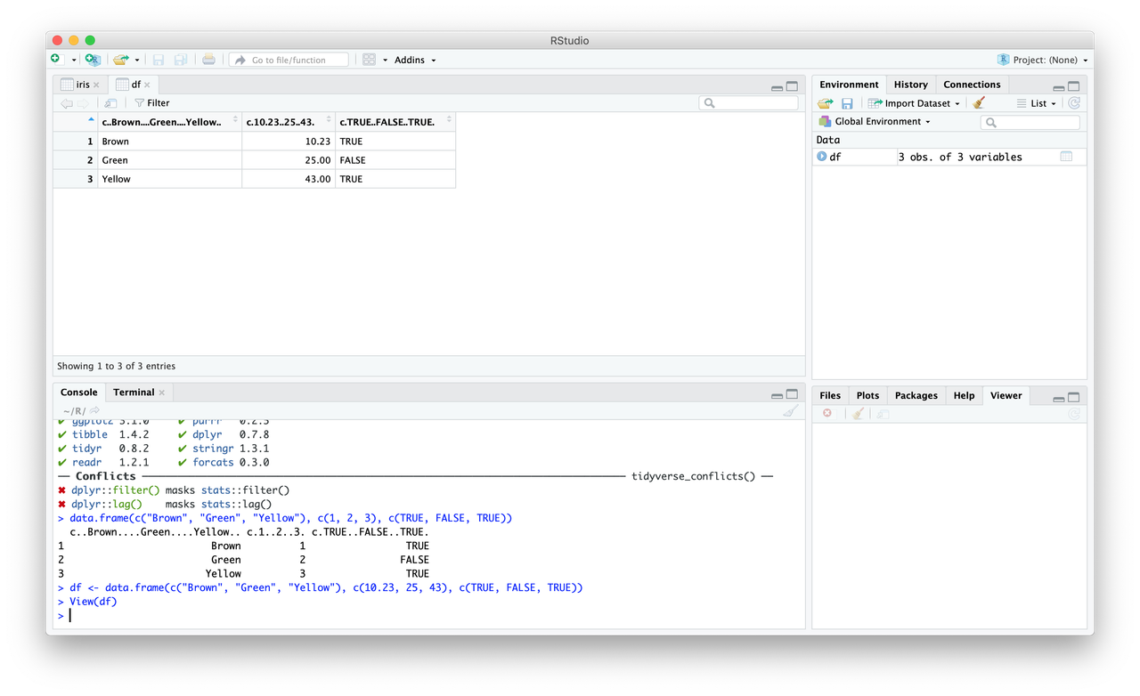
To write a data frame explicitly:
df <- data.frame(c("Brown", "Green", "Yellow"), c(10.23, 25, 43), c(TRUE, FALSE, TRUE)). You’ll notice, however, that the column names are all ugly…colnames(df) <- c("Color", "Some Number", "Dislike")
For now, let’s use the iris database.
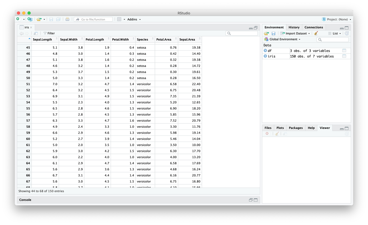
A key reason to use R is to manipulate data with a clear, reproducible trail. Let’s say we want the area of the petals; how would we do this?
There are three parts to this problem: referencing the columns, multiplying the columns, and storing the results.
- In R, reference columns with the
$operator. To find the area, we need to multiply thePetal.Lengthcolumn withPetal.Width - We multiply with the multiplication operator
- We create a new column by referencing it as if it exists
In sum: iris$Petal.Area <- iris$Petal.Length * iris$Petal.Width. Easy, right? There are better ways to do this (using the tidyverse), but we’ll get into those later.
Note: It’s often useful to make column names multiple words when you want a clean output, but it’ll make some manipulation annoying. To refer to these columns, you’ll have to surround their names in back-ticks (e.g.
df$`Some Number`).
Let’s do the same thing for the sepals (whatever the hell that is…): iris$Sepal.Area <- iris$Sepal.Length * iris$Sepal.Width
Let’s say that we only want big plants, so we decide to remove those with sepal areas less than 20. We can crudely filter our data (again, a cleaner way is coming!) with some handy brackets: iris <- iris[iris$Sepal.Area >= 20, ].

There’s quite a bit to break down, starting from the inside and moving out:
- We reference the
Sepal.Areacolumn as we would any other - The greater than or equal to operator (
>=) is the same as in most other languages, as are most other logical operators (e.g.<,==, etc.) - The most perplexing part of this expression is probably the comma. Huh? The brackets are effectively a subset command, and the comma after the expression tells R that you want to filter on the rows. You could also do this on columns—for example, you could remove columns where the maximum value is less than a certain threshold. In that case, you would put the comma right after the opening bracket
- We wrap the inner part in the brackets as a sort of subset of the larger
irisdatabase
Great! The Gender column is pretty useless (how’d that get there? Just don’t ask), so let’s get rid of it. How? Set the column to NULL: iris$Gender <- NULL. All gone!
We now generally know how to read in data, form our own data frame, rename columns, perform simple operations, filter, and remove columns. What should we do with our data?
Plotting
The feature for which R is most famous is the ease and beauty of its plotting. Base graphics are kinda meh, so let’s upgrade to one of the best packages ever written, which should load in when you install and require() the tidyverse: ggplot2.
Let’s create a simple scatter plot between Sepal.Area and Petal.Area: p <- ggplot(iris, aes(x = Petal.Area, y = Sepal.Area)) + geom_point(). p is now the plot object, which you must print: print(p)

And once again, let’s break it down:
ggplot(data, aes())is the first command. Fill indatawith the name of your data frame;aes(), which stands for “aesthetics”, is where you declare your variables (and more—later!). Notice how you don’t need to add theiris$before each column name: This is a really nice feature in thetidyverse, of whichggplot2is part.- In
ggplot2, you “add” the parts of your plot together geom_point()adds… points;geom_bar()will give you a bar graph,geom_boxplot()a boxplot,geom_violin()a violin plot, etc.
Let’s add some more to the plot: p2 <- p + geom_smooth() + ggtitle("What do these things mean"). Don’t forget to print(p2)!

A bit more breakdown:
geom_smooth()adds a curve to fit your data, along with the 95% confidence interval around itggtitle()adds a title to your plot
Some more customization: p3 <- p + geom_smooth(method = "lm", linetype = 2, color = "red", se = FALSE) + labs(x = "Petal", y = "Sepal", title = "Some area stuff", caption = "Not really sure")

What did we do here? Last breakdown of the day:
- The
methodparameter allows us to choose the smoothing method; we chose a line linetypeallows us to change how the line looks, for which there are a bunch of optionscoloris pretty self-explanatorysecontrols the visualization of the confidence interval- The
labs()function works likeggtitle(), but it’s more general
And let’s add a nice theme: p4 <- p3 + nice_theme() + theme(plot.title = element_text(size = 20))

Wrap up
In all honesty, this should be enough to get you through at least the beginning of stat. But R is so much more powerful than just that: Take a look at these examples of interactive web apps, interactive presentations, R markdown webpages (like all my stat homework), and some beautiful graphics; don’t forget some crazy models and nice web scrapping.
No one memorizes all the functions in R, which is why there are a bajillion Stack Overflow questions and answers to which you can look for guidance. Try to simplify your Google search, and you’ll be sure to find something good.
Next week, we’ll explore the tidyverse (better data manipulation) and some more ggplot2 (so many options!!).